In this post we’re going to make a pizza pie… chart. Not as delicious as real pizza, but this is a cool trick to jazz up your charts and involves changing the fill option to a picture for your various data points. This trick works for other charts like bar charts and you don’t have to fill them with a pizza picture, you can use something more relevant to your data, so if you’re an office supply company and you wanted to make a graph showing your top 5 products you could use pictures of pens, pencils, staples, paperclips and paper.
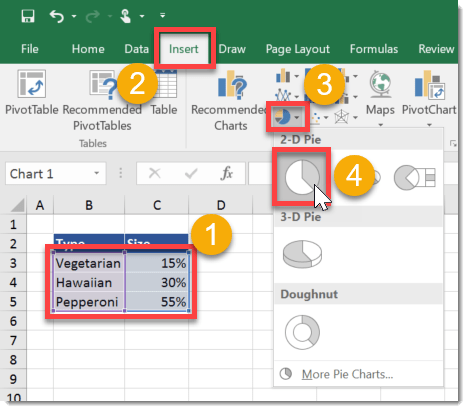
Add a pie chart to your workbook.
Left click on the chart to select it, then left click again on an individual slice of the pie to select that piece. Right click on the selected piece of pie and choose Format Data Point from the menu.
A new Format Data Point window pane will appear on the right.
I added some different pizza pictures for each of the data points. In this case I had three different data points so I added three different pizza pictures for each by repeating the above steps. Bon appetite, a pizza pie chart fresh from the Excel oven!